DataFrame-level Stats Examples#
Basic examples of statistical test methods.
Used Libraries#
The following methods selectively use these libraries:
import plotly.io as pio
pio.renderers.default = "notebook"
Normality Test#
normality() - Tests for normal distribution
from frameon import load_dataset, FrameOn as fo
titanic = fo(load_dataset('titanic'))
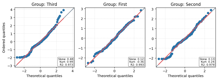
titanic.stats.normality(
dv='age',
between='class',
method='jarque_bera',
show_qqplot=True
)
⚠️ Found 177 (19.87%) missing values in dependent variable 'age'
⚠️ Group 'First' in factor 'class' has 30 (13.89%) missing values in 'age'
⚠️ Group 'Second' in factor 'class' has 11 (5.98%) missing values in 'age'
⚠️ Group 'Third' in factor 'class' has 136 (27.70%) missing values in 'age'
Removed 177 rows (19.87% of data) with missing values in: age, class

Normality Test Report

- Dependent Variable: age
- Grouping Variable: class
- Alpha Level: 0.05
- Test Method: jarque_bera

🔹 Hypothesis Formulation

- H0: The data follows a normal distribution
- H1: The data does not follow a normal distribution
| W | pval | normal | Reject H0 | |
|---|---|---|---|---|
| group | ||||
| Third | 27.48 | 0.00 | False | True |
| First | 1.57 | 0.46 | True | False |
| Second | 0.80 | 0.67 | True | False |
Warning: Non-normal distributions detected in groups: Third
Levene’s Test#
levene() - Tests equality of variances across groups.
from frameon import load_dataset, FrameOn as fo

titanic = fo(load_dataset('titanic'))
titanic.stats.levene(
    dv='age',
    between='class'
)
⚠️ Found 177 (19.87%) missing values in dependent variable 'age'
⚠️ Group 'First' in factor 'class' has 30 (13.89%) missing values in 'age'
⚠️ Group 'Second' in factor 'class' has 11 (5.98%) missing values in 'age'
⚠️ Group 'Third' in factor 'class' has 136 (27.70%) missing values in 'age'
Removed 177 rows (19.87% of data) with missing values in: age, class

Levene's Test Report

- Dependent Variable: age
- Groups: Third vs First
- Alpha Level: 0.05
| W | pval | equal_var | |
|---|---|---|---|
| levene | 5.620164 | 0.003787 | False |
Conclusion: At alpha = 0.05, we reject the null hypothesis that the variances are equal (p=0.0038).
T-Test#
ttest() - Compares means between two groups using independent samples t-test.
from frameon import load_dataset, FrameOn as fo

titanic = fo(load_dataset('titanic'))
titanic.stats.ttest(
    dv='age',
    between='alive',
)
⚠️ Found 177 (19.87%) missing values in dependent variable 'age'
⚠️ Group 'no' in factor 'alive' has 125 (22.77%) missing values in 'age'
⚠️ Group 'yes' in factor 'alive' has 52 (15.20%) missing values in 'age'
Removed 177 rows (19.87% of data) with missing values in: age, alive

T-Test Report

- Dependent Variable: age
- Between Factor: alive (no vs yes)
- Alpha Level: 0.05
- Alternative: two-sided

🔹 Hypothesis Formulation

- H0: The mean of no equals the mean of yes
- H1: The mean of no differs from the mean of yes

🔹 Descriptive Statistics
| Group | count | mean | std | min | max |
|---|---|---|---|---|---|
| no | 424 | 30.63 | 14.17 | 1.0 | 74.0 |
| yes | 290 | 28.34 | 14.95 | 0.42 | 80.0 |
🔹 Homogeneity of Variance (Levene's Test)
| W | pval | equal_var | |
|---|---|---|---|
| levene | 1.195 | 0.275 | True |
- Using Student's t-test - equal variances assumed (pval = 0.275 ≥ 0.05)

🔹 T-Test Results
| T | dof | alternative | p-val | CI95% | cohen-d | BF10 | power | |
|---|---|---|---|---|---|---|---|---|
| T-test | 2.067 | 712 | two-sided | 0.039 | [0.11 4.45] | 0.157 | 0.685 | 0.541 |
🔹 Conclusion: At alpha = 0.05, we reject the null hypothesis (p-val = 0.0391).
Mann-Whitney U Test#
mwu() - Non-parametric test for comparing two independent groups.
from frameon import load_dataset, FrameOn as fo

titanic = fo(load_dataset('titanic'))
titanic.stats.mwu(
    dv='age',
    between='alive'
)
⚠️ Found 177 (19.87%) missing values in dependent variable 'age'
⚠️ Group 'no' in factor 'alive' has 125 (22.77%) missing values in 'age'
⚠️ Group 'yes' in factor 'alive' has 52 (15.20%) missing values in 'age'
Removed 177 rows (19.87% of data) with missing values in: age, alive

Mann-Whitney U Test Report

- Dependent Variable: age
- Between Factor: alive (no vs yes)
- Alpha Level: 0.05
- Alternative: two-sided

🔹 Hypothesis Formulation

- H0: The distribution of no equals the distribution of yes
- H1: The distribution of no differs from the distribution of yes

🔹 Descriptive Statistics
| Group | count | median | mean | std | min | max |
|---|---|---|---|---|---|---|
| no | 424 | 28.0 | 30.63 | 14.17 | 1.0 | 74.0 |
| yes | 290 | 28.0 | 28.34 | 14.95 | 0.42 | 80.0 |
🔹 Mann-Whitney U Test Results
| U-val | alternative | p-val | RBC | CLES | |
|---|---|---|---|---|---|
| MWU | 65278.0 | two-sided | 0.16 | 0.062 | 0.531 |
Effect Sizes:
- Rank-Biserial Correlation (RBC) = 0.06 (small effect)
- Common Language Effect Size (CLES) = 0.53 (small effect)

🔹 Conclusion: At alpha = 0.05, we fail to reject the null hypothesis (p-val = 0.1605).
ANOVA#
anova() - One-way analysis of variance for comparing means across multiple groups.
from frameon import load_dataset, FrameOn as fo

titanic = fo(load_dataset('titanic'))
titanic.stats.anova(
    dv='age',
    between='class'
)
⚠️ Found 177 (19.87%) missing values in dependent variable 'age'
⚠️ Group 'First' in factor 'class' has 30 (13.89%) missing values in 'age'
⚠️ Group 'Second' in factor 'class' has 11 (5.98%) missing values in 'age'
⚠️ Group 'Third' in factor 'class' has 136 (27.70%) missing values in 'age'
Removed 177 rows (19.87% of data) with missing values in: age, class

One-way ANOVA Report

- Dependent Variable: age
- Between Factors: class
- Alpha Level: 0.05

🔹 Hypothesis Formulation

- H0: All group means are equal (Third, First, Second)
- H1: At least one group mean differs among Third, First, Second

🔹 Descriptive Statistics
| Group | count | mean | std | min | max | median |
|---|---|---|---|---|---|---|
| First | 186 | 38.23 | 14.8 | 0.92 | 80.0 | 37.0 |
| Second | 173 | 29.88 | 14.0 | 0.67 | 70.0 | 29.0 |
| Third | 355 | 25.14 | 12.5 | 0.42 | 74.0 | 24.0 |
🔹 Homogeneity of Variance Check
| W | pval | equal_var | |
|---|---|---|---|
| levene | 5.62 | 0.004 | False |
- Using Welch's ANOVA - Levene's test showed unequal variances (pval = 0.004 < 0.05)

🔹 Welch ANOVA Results
| Source | ddof1 | ddof2 | F | p-unc | np2 |
|---|---|---|---|---|---|
| class | 2 | 359.444 | 53.355 | 0.0 | 0.139 |
🔹 Post-hoc Analysis
| A | B | mean(A) | mean(B) | diff | se | T | df | pval | hedges |
|---|---|---|---|---|---|---|---|---|---|
| First | Second | 38.233 | 29.878 | 8.356 | 1.52 | 5.496 | 356.897 | 0.0 | 0.578 |
| First | Third | 38.233 | 25.141 | 13.093 | 1.272 | 10.293 | 325.228 | 0.0 | 0.981 |
| Second | Third | 29.878 | 25.141 | 4.737 | 1.254 | 3.777 | 308.829 | 0.001 | 0.364 |
🔹 Conclusion: Significant effects found (p-unc = 0.000)

Significant pairwise comparisons:
- First vs Second: pval = 0.000
- First vs Third: pval = 0.000
- Second vs Third: pval = 0.001
Kruskal-Wallis Test#
kruskal() - Non-parametric alternative to one-way ANOVA.
from frameon import load_dataset, FrameOn as fo

titanic = fo(load_dataset('titanic'))
titanic.stats.kruskal(
    dv='age',
    between='class'
)
⚠️ Found 177 (19.87%) missing values in dependent variable 'age'
⚠️ Group 'First' in factor 'class' has 30 (13.89%) missing values in 'age'
⚠️ Group 'Second' in factor 'class' has 11 (5.98%) missing values in 'age'
⚠️ Group 'Third' in factor 'class' has 136 (27.70%) missing values in 'age'
Removed 177 rows (19.87% of data) with missing values in: age, class

Kruskal-Wallis Test Report

- Dependent Variable: age
- Grouping Variable: class
- Groups: Third, First, Second
- Alpha Level: 0.05

🔹 Hypothesis Formulation

- H0: The distributions of all groups are equal (Third, First, Second)
- H1: At least one group distribution differs among Third, First, Second

🔹 Descriptive Statistics
| Group | count | median | mean | std | min | max |
|---|---|---|---|---|---|---|
| First | 186 | 37.0 | 38.23 | 14.8 | 0.92 | 80.0 |
| Second | 173 | 29.0 | 29.88 | 14.0 | 0.67 | 70.0 |
| Third | 355 | 24.0 | 25.14 | 12.5 | 0.42 | 74.0 |
🔹 Kruskal-Wallis Test Results
| Source | ddof1 | H | p-unc |
|---|---|---|---|
| class | 2 | 95.995 | 0.0 |
🔹 Post-hoc Analysis (Dunn's Test)
| A | B | p-corr |
|---|---|---|
| First | Second | 0.0 |
| First | Third | 0.0 |
| Second | Third | 0.0 |
🔹 Conclusion: Significant difference found (p-unc = 0.000)

Significant pairwise comparisons:
- First vs Second: pval = 0.000
- First vs Third: pval = 0.000
- Second vs Third: pval = 0.000
Chi-Square Test#
chi2_independence() - Tests categorical variable independence
from frameon import load_dataset, FrameOn as fo

titanic = fo(load_dataset('titanic'))
titanic.stats.chi2_independence(
    x='class',
    y='alive',
    test='pearson'
)
Categorical Association Report

- class vs alive
- Total observations: 891


🔹 Hypothesis Formulation

- H0: class and alive are independent (Third, First, Second vs no, yes)
- H1: class and alive are associated (Third, First, Second vs no, yes)

🔹 Contingency Table
| alive | no | yes |
|---|---|---|
| class | ||
| First | 80 | 136 |
| Second | 97 | 87 |
| Third | 372 | 119 |
🔹 Statistical Tests
| test | lambda | chi2 | dof | pval | cramer | power | cramer strength |
|---|---|---|---|---|---|---|---|
| pearson | 1.0 | 102.889 | 2.0 | 0.0 | 0.34 | 1.0 | Moderate |
🔹 Conclusion: At alpha = 0.05, we reject the null hypothesis of independence (pearson test, p = 0.000).
No significant association found between class and alive.
Bootstrap#
bootstrap() - Computes bootstrap confidence intervals
from frameon import load_dataset, FrameOn as fo

titanic = fo(load_dataset('titanic'))
titanic.stats.bootstrap(
    dv='age',
    between='alive',
    reference_group='no',
    statistic='mean_diff',
    plot=True
)
⚠️ Found 177 (19.87%) missing values in dependent variable 'age'
⚠️ Group 'no' in factor 'alive' has 125 (22.77%) missing values in 'age'
⚠️ Group 'yes' in factor 'alive' has 52 (15.20%) missing values in 'age'
Removed 177 rows (19.87% of data) with missing values in: age, alive
| method | statistic | n_resamples | standard_error | ci | alternative |
|---|---|---|---|---|---|
| BCa | 2.28 | 9999 | 1.11 | [0.11, 4.50] | two-sided |
Linear Regression#
ols() - Ordinary least squares regression
from frameon import load_dataset, FrameOn as fo
diamonds = fo(load_dataset('diamonds'))
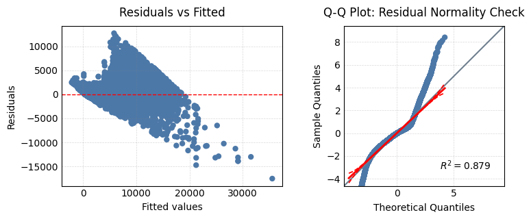
diamonds.stats.ols(
formula='price ~ carat + C(cut, Treatment("Ideal"))',
cov_type='HC3',
show_plots=True
)
| Variable | VIF |
|---|---|
| carat | 2.08 |
| C(cut, Treatment("Ideal"))[T.Premium] | 1.491 |
| C(cut, Treatment("Ideal"))[T.Very Good] | 1.352 |
| C(cut, Treatment("Ideal"))[T.Good] | 1.158 |
| C(cut, Treatment("Ideal"))[T.Fair] | 1.079 |
                            OLS Regression Results
==============================================================================
Dep. Variable:                  price   R-squared:                       0.856
Model:                            OLS   Adj. R-squared:                  0.856
Method:                 Least Squares   F-statistic:                 2.092e+04
Date:                Thu, 31 Jul 2025   Prob (F-statistic):               0.00
Time:                        11:12:31   Log-Likelihood:            -4.7142e+05
No. Observations:               53940   AIC:                         9.429e+05
Df Residuals:                   53934   BIC:                         9.429e+05
Df Model:                           5
Covariance Type:                  HC3
===========================================================================================================
                                              coef    std err          t      P>|t|      [0.025      0.975]
-----------------------------------------------------------------------------------------------------------
Intercept                               -2074.5457     16.092   -128.920      0.000   -2106.086   -2043.006
C(cut, Treatment("Ideal"))[T.Fair]      -1800.9240     51.723    -34.819      0.000   -1902.301   -1699.547
C(cut, Treatment("Ideal"))[T.Good]       -680.5921     22.873    -29.755      0.000    -725.423    -635.761
C(cut, Treatment("Ideal"))[T.Premium]    -361.8468     17.209    -21.026      0.000    -395.577    -328.116
C(cut, Treatment("Ideal"))[T.Very Good]  -290.7886     16.684    -17.430      0.000    -323.488    -258.089
carat                                    7871.0821     24.892    316.207      0.000    7822.293    7919.871
==============================================================================
Omnibus:                    14616.138   Durbin-Watson:                   1.027
Prob(Omnibus):                  0.000   Jarque-Bera (JB):           150962.278
Skew:                           1.007   Prob(JB):                         0.00
Kurtosis:                      10.944   Cond. No.                         8.39
==============================================================================

Notes:
[1] Standard Errors are heteroscedasticity robust (HC3)
Robust Linear Model#
rlm() - Regression with robust standard errors
from frameon import load_dataset, FrameOn as fo

diamonds = fo(load_dataset('diamonds'))
diamonds.stats.rlm(
    formula='price ~ carat + C(cut, Treatment("Ideal"))',
)
| Variable | VIF |
|---|---|
| carat | 2.08 |
| C(cut, Treatment("Ideal"))[T.Premium] | 1.491 |
| C(cut, Treatment("Ideal"))[T.Very Good] | 1.352 |
| C(cut, Treatment("Ideal"))[T.Good] | 1.158 |
| C(cut, Treatment("Ideal"))[T.Fair] | 1.079 |
                    Robust linear Model Regression Results
==============================================================================
Dep. Variable:                  price   No. Observations:                53940
Model:                            RLM   Df Residuals:                    53934
Method:                          IRLS   Df Model:                            5
Norm:                          HuberT
Scale Est.:                       mad
Cov Type:                          H1
Date:                Thu, 31 Jul 2025
Time:                        11:12:32
No. Iterations:                    23
===========================================================================================================
                                              coef    std err          z      P>|z|      [0.025      0.975]
-----------------------------------------------------------------------------------------------------------
Intercept                               -1834.9416      8.689   -211.172      0.000   -1851.972   -1817.911
C(cut, Treatment("Ideal"))[T.Fair]      -1263.4005     24.022    -52.593      0.000   -1310.483   -1216.318
C(cut, Treatment("Ideal"))[T.Good]       -490.9289     14.651    -33.507      0.000    -519.645    -462.213
C(cut, Treatment("Ideal"))[T.Premium]    -231.6302     10.192    -22.727      0.000    -251.606    -211.654
C(cut, Treatment("Ideal"))[T.Very Good]  -220.2565     10.525    -20.926      0.000    -240.886    -199.627
carat                                    7219.3427      8.535    845.812      0.000    7202.614    7236.072
===========================================================================================================

If the model instance has been used for another fit with different fit parameters, then the fit options might not be the correct ones anymore .
Generalized Linear Model#
glm() - Generalized linear regression
from frameon import load_dataset, FrameOn as fo
import statsmodels.api as sm

titanic = fo(load_dataset('titanic'))
titanic.stats.glm(
    formula='survived ~ age + sex + pclass',
    family=sm.families.Binomial()
)
| Variable | VIF |
|---|---|
| pclass | 3.359 |
| age | 2.924 |
| sex[T.male] | 2.859 |
                 Generalized Linear Model Regression Results
==============================================================================
Dep. Variable:               survived   No. Observations:                  714
Model:                            GLM   Df Residuals:                      710
Model Family:                Binomial   Df Model:                            3
Link Function:                  Logit   Scale:                          1.0000
Method:                          IRLS   Log-Likelihood:                -323.65
Date:                Thu, 31 Jul 2025   Deviance:                       647.29
Time:                        11:12:32   Pearson chi2:                     768.
No. Iterations:                     5   Pseudo R-squ. (CS):             0.3587
Covariance Type:                  HC3
===============================================================================
                  coef    std err          t      P>|t|      [0.025      0.975]
-------------------------------------------------------------------------------
Intercept       5.0560      0.526      9.607      0.000       4.023       6.089
sex[T.male]    -2.5221      0.203    -12.444      0.000      -2.920      -2.124
age            -0.0369      0.008     -4.610      0.000      -0.053      -0.021
pclass         -1.2885      0.148     -8.718      0.000      -1.579      -0.998
===============================================================================
Quantile Regression#
quantreg() - Quantile regression
from frameon import load_dataset, FrameOn as fo

diamonds = fo(load_dataset('diamonds'))
diamonds.stats.quantreg(
    formula='price ~ carat + C(cut, Treatment("Ideal"))',
    q=0.95
)
| Variable | VIF |
|---|---|
| carat | 2.08 |
| C(cut, Treatment("Ideal"))[T.Premium] | 1.491 |
| C(cut, Treatment("Ideal"))[T.Very Good] | 1.352 |
| C(cut, Treatment("Ideal"))[T.Good] | 1.158 |
| C(cut, Treatment("Ideal"))[T.Fair] | 1.079 |
                         QuantReg Regression Results
==============================================================================
Dep. Variable:                  price   Pseudo R-squared:               0.7297
Model:                       QuantReg   Bandwidth:                       220.4
Method:                 Least Squares   Sparsity:                        6958.
Date:                Thu, 31 Jul 2025   No. Observations:                53940
Time:                        11:12:32   Df Residuals:                    53934
                                        Df Model:                            5
===========================================================================================================
                                              coef    std err          t      P>|t|      [0.025      0.975]
-----------------------------------------------------------------------------------------------------------
Intercept                               -2220.0986     14.000   -158.574      0.000   -2247.540   -2192.658
C(cut, Treatment("Ideal"))[T.Fair]       -886.8169     40.760    -21.757      0.000    -966.707    -806.927
C(cut, Treatment("Ideal"))[T.Good]       -291.6197     24.700    -11.807      0.000    -340.031    -243.208
C(cut, Treatment("Ideal"))[T.Premium]    -102.2676     17.318     -5.905      0.000    -136.211     -68.325
C(cut, Treatment("Ideal"))[T.Very Good]   137.0000     17.739      7.723      0.000     102.231     171.769
carat                                    1.063e+04     16.741    635.114      0.000    1.06e+04    1.07e+04
===========================================================================================================
Ordered Model#
ordered_model() - Regression for ordered categorical dependent variables.
from frameon import load_dataset, FrameOn as fo
import pandas as pd

diamonds = fo(load_dataset('diamonds'))
cut_order = ['Fair', 'Good', 'Very Good', 'Premium', 'Ideal']
diamonds['cut'] = pd.Categorical(diamonds['cut'], categories=cut_order, ordered=True)
diamonds.stats.ordered_model(
    formula='cut ~ carat + price',
    distr='logit'
)
Optimization terminated successfully.
         Current function value: 1.349193
         Iterations: 28
         Function evaluations: 33
         Gradient evaluations: 33
                             OrderedModel Results
==============================================================================
Dep. Variable:                    cut   Log-Likelihood:                -72775.
Model:                   OrderedModel   AIC:                         1.456e+05
Method:            Maximum Likelihood   BIC:                         1.456e+05
Date:                Thu, 31 Jul 2025
Time:                        11:12:34
No. Observations:               53940
Df Residuals:                   53934
Df Model:                           2
=====================================================================================
                        coef    std err          z      P>|z|      [0.025      0.975]
-------------------------------------------------------------------------------------
carat                -2.1468      0.045    -47.500      0.000      -2.235      -2.058
price                 0.0002   5.37e-06     38.579      0.000       0.000       0.000
Fair/Good            -4.4558      0.033   -136.610      0.000      -4.520      -4.392
Good/Very Good        0.4227      0.015     28.551      0.000       0.394       0.452
Very Good/Premium     0.3132      0.009     36.365      0.000       0.296       0.330
Premium/Ideal         0.0793      0.008     10.283      0.000       0.064       0.094
=====================================================================================
Mixed Linear Model#
mixedlm() - Linear regression with random effects.
from frameon import load_dataset, FrameOn as fo

penguins = fo(load_dataset('penguins'))
penguins.stats.mixedlm(
    "body_mass_g ~ bill_length_mm + C(sex)",
    groups="island"
)
| Variable | VIF |
|---|---|
| bill_length_mm | 2.173 |
| C(sex)[T.MALE] | 2.173 |
              Mixed Linear Model Regression Results
=================================================================
Model:                MixedLM   Dependent Variable:   body_mass_g
No. Observations:     333       Method:               REML
No. Groups:           6         Scale:                0.0000
Min. group size:      1         Log-Likelihood:       2410.1918
Max. group size:      1         Converged:            Yes
Mean group size:      1.0
-----------------------------------------------------------------
                Coef.    Std.Err.    z    P>|z|  [0.025   0.975]
-----------------------------------------------------------------
Intercept      3876.707    330.617 11.726 0.000 3228.709 4524.705
C(sex)[T.MALE]  171.865     19.946  8.617 0.000  132.771  210.958
bill_length_mm   -8.892      8.505 -1.046 0.296  -25.562    7.777
Group Var       518.642 279357.703
=================================================================
Feature Importance Analysis#
feature_importance_analysis() - Analyzes feature importance for data analysis.
from frameon import load_dataset, FrameOn as fo

iris = fo(load_dataset('iris'))
iris.stats.feature_importance_analysis(
    target_column='species',
    feature_columns=iris.columns.difference(['species', 'species_id']).tolist()
)